Disabling Screen Updates in Excel VBA

One quick and easy technique to make your code run faster in Excel VBA is to simply prevent the screen from being redrawn each time something changes.  You can achieve this by using the ScreenUpdating property of the Application object.

Creating a Simple Example

To demonstrate the principle of this technique we'll need a small example procedure that makes lots of visible changes to the Excel workbook.  You can either download the example here, or create a new blank workbook, add around five worksheets to it and then copy the code shown below into a new module.

Running the Code with Screen Updates On

Before disabling screen updates it's worth running the code with the property switched on so that you can appreciate the difference.  Head back into Excel and either press ALT + F8 on the keyboard or, from the ribbon select Developer | Macros.  On the dialog box that appears select the ColourInABunchOfCells macro and then click the Run button.

Select the macro and then click Run.

You should be able to see the Excel screen flickering in the background as the macro carries out its tasks until, eventually, it finishes.

Disabling Screen Updates

The next time we run the procedure we don't want to be able to see the screen flickering in the background.  To achieve this we need to add a single line of code to the subroutine, just below the variable declarations.  It's probably also worth changing the colour that we're using so that we can see when things have changed.

Now switch back to Excel, display the list of macros by pressing ALT + F8 and then run the code again.  This time you won't be able to see the macro carrying out its tasks; once the subroutine has finished the screen will update once at the end to show you the final result.

Adding a Basic Timer

You may have noticed that when running the procedure with screen updates disabled the subroutine appeared to run faster.  This should certainly be the case as Excel doesn't have to continually redraw the screen each time something changes.  If we want to quantify how much time we've saved we can add some code to create a basic timer system.  The general structure of our timer is shown below:

Adding this timer system to our colour macro should result in the following code:

When you run the subroutine again you should now see the time taken in seconds displayed at the end of the procedure.  You should test this both with and without screen updating to determine how much faster your code runs.

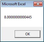
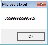
Running the code with screen updates turned on takes just over 8 seconds.	Running the macro with screen updates disabled takes just less than 1 second.

Your results will vary depending on your computer's specifications and a range of other factors but you should certainly see an improvement in performance when screen updates are turned off.

A More Complex Example

Although the example above demonstrates the principle of the technique, it doesn't really reflect the type of code you're likely to write in the real world.  The example below is slightly more realistic.  The basic idea behind this example is to separate a list of films into separate worksheets based on each film's genre.

The idea is to create a separate worksheet for each genre and copy each film into the appropriate sheet.

You can download the completed example file here and the code is shown below for your reference.

There's also a simple routine that you can run to reset the workbook back to the original state by deleting all of the genre worksheets.

Again, to test the performance gain you should run the code with screen updates turned on and then turned off.

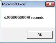
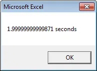
With screen updates turned on the procedure takes almost 7 seconds.	Without screen updates the code takes just less than 2 seconds.

An Alternative Approach: Avoiding Selecting Things

Although you can save a lot of time by turning screen updates off, you can also find performance gains by writing your code in such a way that Excel needs to update the screen as little as possible.  The easiest way to achieve this to avoid selecting or activating objects such as worksheets and ranges as much as possible.  In the example code shown below the only time an object is selected is when a new worksheet is added to the workbook.

Running this code even with screen updates turned on results in the following time:

This code runs quickly even with screen updates turned on.