Read our blogs, tips and tutorials
Try our exercises or test your skills
Watch our tutorial videos or shorts
Take a self-paced course
Read our recent newsletters
License our courseware
Book expert consultancy
Buy our publications
Get help in using our site
546 attributed reviews in the last 3 years
Refreshingly small course sizes
Outstandingly good courseware
Whizzy online classrooms
Wise Owl trainers only (no freelancers)
Almost no cancellations
We have genuine integrity
We invoice after training
Review 30+ years of Wise Owl
View our top 100 clients
Search our website
We also send out useful tips in a monthly email newsletter ...
How to add sparklines to Excel cells to show trends (and options for formatting) |
---|
Learn how to get individual Excel cells to contain sparklines to show trends, how to display column charts or win/loss charts instead, how to play about with grouped charts, how to change sparkline formatting and how to customise sparkline axes. |
In this blog
Sparklines have been around in Excel for some time now, but are easily forgotten (not least by me!).
I thought I'd show how you can quickly apply them to cells to illustrate trends.
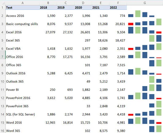
Skills assessment tests taken on the Wise Owl site in the last 5 complete years, showing the low (red) and high (green) point for each subject.
If you want to follow along you can easily do so - just download and unzip this Excel file.
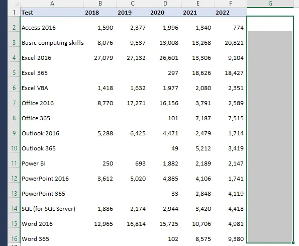
Start by selecting the cell or cells in which to put your sparklines:
An alternative strategy would be to create a sparkline for the top cell (Access 2016 in this case) and then copy it down to the cells beneath it.
Now choose to insert a sparkline:
You can add a line, column or win/loss sparkline (see later in this blog for what the a win/loss sparkline might look like).
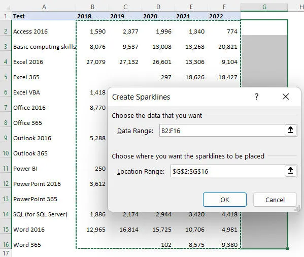
Choose your data range, then select OK:
Here we've chosen to get data from the rows to the left of each sparkline cell.
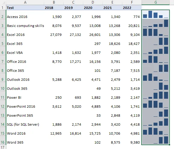
You should now have some sparklines:
I chose to add column sparklines, so strictly speaking I guess I've got sparkbars.
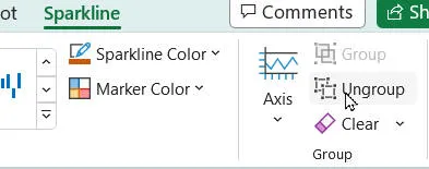
When you add sparklines like this, they will be grouped:
If you want to format each sparkline separately, you can - you will first need to choose this option to ungroup them.
You'd be unlikely to want to ungroup these sparklines: it's convenient that you can change the formatting of one of them and have the others automatically update at the same time.
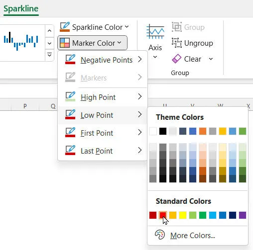
The easiest way to change the colour of the maximum and minimum value in each sparkline is like this:
Choose the options shown to change the low point or high point colours.
Note that when you do this Excel will automatically tick the appropriate options:
These boxes have been ticked automatically.
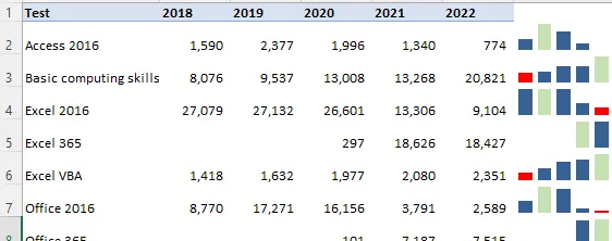
It's now much easier to pick out trends:
You can clearly see that fewer people are taking our Access 2016 test, but many more the basic computing skills test.
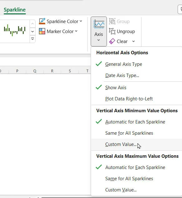
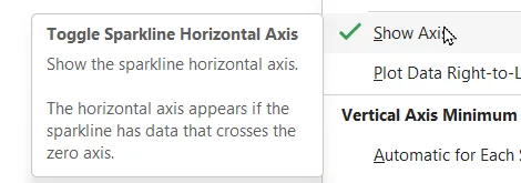
Excel will usually set the axis of a sparkline to start at 0, but sometimes this can give misleading results. To change this, go to the Axis dropdown in the dedicated sparkline ribbon:
Here I've chosen to show the axis, and am about to change the minimum value.
Now type in a new custom minimum value:
Values below 1,000 now won't be shown.
On this occasion this change hasn't made anything clearer!
The revised chart: values below 1,000 have disappeared.
Here's why we don't get an axis for our sparklines, even though we asked for one:
I THINK this makes sense!
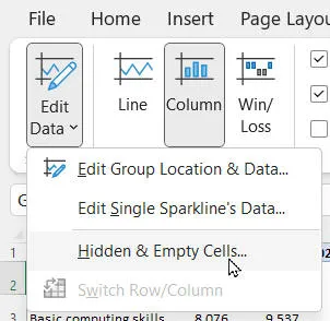
Where you have gaps in your data, here's how to specify how they should be treated. First go to the relevant dialog box:
Choose this option to decide how to show empty and hidden cells.
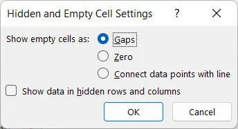
You can then choose which option you want to apply:
See below to see the effect given by each of these options.
Here's an example of each option:
I've added in an extra value for Excel 365 tests for year 1. The first option fills in any gaps between this and the rest of the data, the second option displays missing points as zeros and the third option connects data points across the missing years.
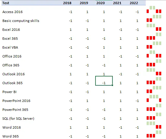
Win/loss charts show binary day. For our example, I've changed the data to show a 1 where the number of tests done was more than the 5-year average, and a -1 otherwise:
The formula I used for the top left cells (Access 2016 tests for 2018) was =IF(B2>AVERAGE($B2:$F2),1,-1).
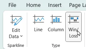
I've changed the sparklines to show win/loss data:
The chart type used in the screenshot above.
I suppose this does show clearly a trend of how you've succeeded or failed over time, but it does seem a bit niche ...
Just for fun, here is Preston North End's win/loss chart in the Championship for the season to date at the time of writing:
Although I've hidden most of the rows, I've configured the win/loss chart to display hidden rows. The chart shows no clear pattern (a bit like Preston, really).
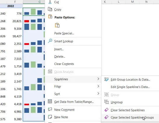
To delete sparklines from a cell you can't just press the Del key. Instead:
To delete sparklines from a cell first right-click on it and then choose one of the Clear options shown above.
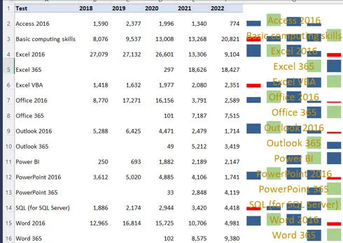
Surprisingly, cells which contain sparklines can also contain text:
Just because you can do something, it doesn't mean you should!
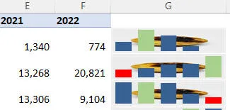
Of course if you wanted to be silly you could use the new IMAGE function in Excel to display images and sparklines in the same cell:
A pastel de nata and a sparkline co-existing unhappily.
And with that I've clearly scraped the bottom of the sparkline barrel!
Some other pages relevant to the above blog include:
Kingsmoor House
Railway Street
GLOSSOP
SK13 2AA
Landmark Offices
99 Bishopsgate
LONDON
EC2M 3XD
Holiday Inn
25 Aytoun Street
MANCHESTER
M1 3AE
© Wise Owl Business Solutions Ltd 2025. All Rights Reserved.