Pivot tables have long been Excel's best tool for grouping and aggregating a large list of data. Consider the following list of movies:

The list contains thousands of films.

You could use a pivot table to divide the films into different groups and calculate statistics for the films in each group:

This pivot table groups the films into different Genres and Certificates and calculates the Average Box Office.

It requires only a few clicks to create the pivot table shown above, but Excel now provides a pair of functions which could make it even faster to summarise your data!

The GROUPBY Function

The GROUPBY function allows you to create a vertical list of groups and calculate a value for the items in each group. Here's the syntax of the function:

Creating a basic set of groups is easier than the above syntax suggests! Only the first three parameters are compulsory:

You can see a simple example in the screenshot below:

This groups by the values in column M and takes the AVERAGE of the values in column D.

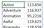
You can see the results of the formula below:

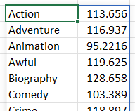
The first few rows returned by the formula.

Choosing Aggregation Functions

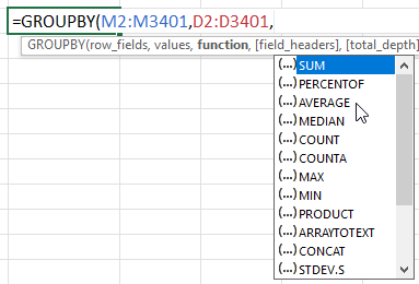
The GROUPBY function makes it easy to choose which function to apply to your data by providing a list of options when you reach that part of your formula.

When you reach the function parameter you can select from a list of options.

Including Column Headers

You can include column headers in the result by using the field_headers parameter. To do this, you must include the headers in the range of cells you provide to the row_fields and values parameters.

The column headers for our list of films are in row 1 of the worksheet.

In the example below, we're choosing to include column headers in the results of the formula:

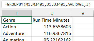
We've included row 1 in the ranges and we're setting the field_headers parameter to a value of 3.

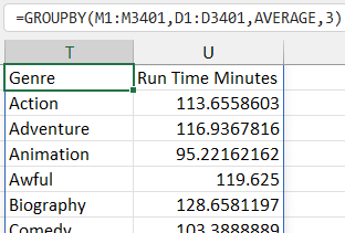
The result of the formula now includes column headers:

A bit of extra formatting would help to make things more readable.

Sorting the Results

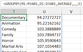
By default, the GROUPBY function sorts the results in ascending order of the first column. You can change this by entering the number of the column you want to sort by in the sort_order parameter. You can use a positive number to sort the column in ascending order:

The number 2 tells the function to sort in ascending order of the second column.

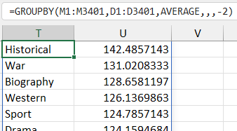
You can use a negative number to sort in descending order:

The number -2 sorts in descending order of the second column of results.

Multiple Calculation Columns

You can refer to multiple columns in the values argument to produce multiple columns of calculations in the output. This is easiest to do with adjacent columns.

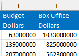
I'd like to aggregate the values of these two columns.

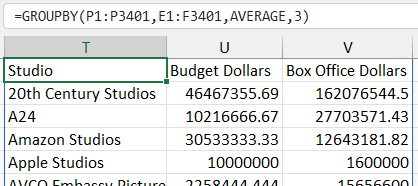
The example below aggregates the values in columns E and F, grouping by the values in column P:

Each column referenced in the values argument produces a separate column in the results.

Aggregating non-adjacent columns is trickier:

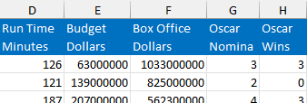
I'd like to find the average of columns D, F and H only.

If we include the full range of cells, the output includes columns that I don't want.

This includes columns that I don't want to see.

Instead, use the CHOOSECOLS function to specify the numbers of the columns in values range.

I've used the CHOOSECOLS function to return columns 1, 3 and 5 from range D1:H3401.

Applying Multiple Functions

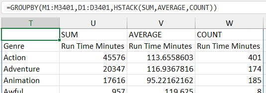
Rather than applying the same function to multiple different columns, you can apply multiple different functions to the same column. You'll need some help from the VSTACK or HSTACK functions to present the results:

Using HSTACK arranges the requested functions horizontally.

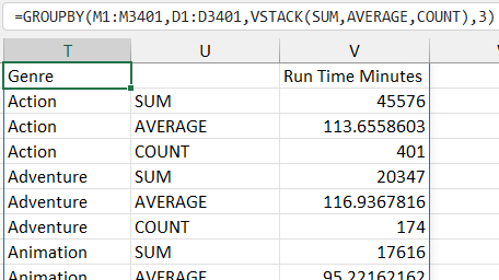
If you prefer to arrange the results vertically, use the VSTACK function:

The VSTACK function creates a row for each function you requested.

Grouping by Multiple Columns

You can use similar techniques to group by multiple columns.

I'd like to group the results by the Genre and Certificate.

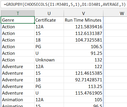
Again, you can use the CHOOSECOLS function to specify which columns you want to pick from a range:

I've used CHOOSECOLS to pick columns 5 and 1 from the range I1:M4301.

Totals and Subtotals

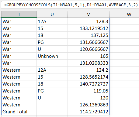
You can use the total_depth parameter to show totals and subtotals.

You can pick from a range of options for displaying totals and subtotals.

You can see the results of the formula in the diagram below:

A subtotal appears below each group, and a grand total appears at the bottom of the table.

Filtering the Data

You can use the filter_array parameter to control which rows are included in the aggregations. In the example below, we're showing the average run time for films grouped by genre:

These results include every film from the list.

Now I'd like to show the same aggregation but only for Oscar-winning films:

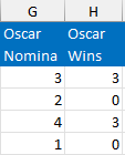
I want to include only films with at least one Oscar Win.

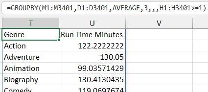
To do this, add a filter to the filter_array parameter. In the example below the filter is H1:H3401>=1:

Notice that at least one genre has disappeared, indicating that there are no Oscar-winning films in that group.

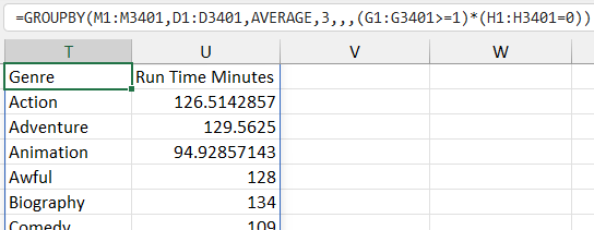
You can combine filters by either multiplying or adding filter expressions. In the example below we're including films with at least 1 Oscar nomination and 0 Oscar wins:

Multiplying filters combines them with AND logic.

In the example below we're including films which made at least $1,000,000,000 at the box office or received at least 10 Oscar nominations:

Adding filters combines them with OR logic.

Using Tables and Structured References

You may find it easier to use the GROUPBY and PIVOTBY functions if you convert your data into a formal Excel table first. To do this, select any cell in the list and from the ribbon choose Insert | Table (or press Ctrl + T on your keyboard).

Click OK to finish creating the table.

After creating the table, it's a good idea to give it a sensible name. You can do this in the Table Design tab of the ribbon.

We've called our table Films.

You can now use structured references to refer to the columns of the table, making the formula easier to understand.

The syntax of a structured reference is Table_name[Column_name]

You can see the results of the formula in the diagram below:

Unfortunately, structured references don't include the column headers from the table.

Summary

The GROUPBY function is perfect for creating row groups and aggregating data in those groups, but what if you want to create both row and column groups? The next part of this blog explains how to use the PIVOTBY function.